© 2005 The American Physical Society
Hideaki Shimazaki
Department of Physics, Graduate School of Science, Kyoto University, Kyoto 606-8502, Japan
Ernst Niebur
Department of Neuroscience, Zanvyl Krieger Mind/Brain Institute, School of Medicine, Johns Hopkins University, Baltimore, Maryland 21218
Competition occurs when two or more players such as organisms, individuals or companies strive for common but limited resources. It plays a significant role in biological and social activities, and is the basis of evolution. Most natural competition processes allow the introduction of new players, which is a hallmark of an open, nonequilibrium system. In this contribution, we introduce an irreversible discrete multiplicative process with normalization at each time step as a generic model of competition. Players with different abilities successively join the game and compete for finite resources. The model shows macroscopically observable changes in its behavior; at a singularity in the statistical distribution of the players' abilities, certain players become dominant over all others. The emergence of dominant players and the evolutionary development of the system occur as a transition from stationary to nonstationary state of the multiplicative process. We analyze the phase transition in the mathematical framework of Bose-Einstein condensation (BEC), although, of course, systems modelled are classical and not quantum mechanical. The same approach has been applied successfully to models of complex networks [Bianconi and Barabasi(2001)] and ecosystems [Volkov et al.(2004)Volkov, Banavar, and Maritan] that behave analogously to a Bose gas. We show that this approach is applicable to bacterial competition, providing surprising insights and predictions to their dynamics.
Before we present the model, we first introduce a general framework for how
our multiplicative competition model is related to a statistical mechanics concept.
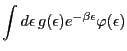
Let
![]() be a function that satisfies the following conditions
for an arbitrary
be a function that satisfies the following conditions
for an arbitrary ![]() density function
density function
![]() defined on
defined on
![]() ,
,
The competition we introduce is defined by three conditions at each time
step.
(i) Players compete for a fixed total amount of resources.
(ii) The resource gained by a player is proportional to the player's innate
ability and to its resource gained at the previous time step.
(iii) New players join the game, each with the same initial resources. The
only exception is the first player (pioneer), who starts the game with all
the resources available.
These rules are summarized in a simple multiplicative process,
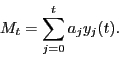
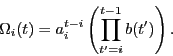
We now consider the time evolution of players except for the pioneer. The
gain of the ![]() th player at time
th player at time ![]() is given by
is given by
![]() , where
, where
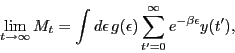
To study this prediction, we simulate the multiplicative process
Eq. 7, adopting a standard density function,
We verified the existence of a BEC analogue in a discrete multiplicative process,
as was shown in a continuous model [Bianconi and Barabasi(2001)]. However, we emphasize
that, as a matter of principle, our classical dynamical system is not equivalent
to a quantum gas. The most important difference is based on the following observation.
The time evolution of each player's gain is different above and below the predicted
![]() . Above
. Above ![]() , the gains of all players monotonically decrease. Below
, the gains of all players monotonically decrease. Below ![]() , not all of them show monotonic behavior, and the competitive dynamics
is disordered. The observed nonequilibrium phase transition from ordered to
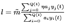
disordered state occurs as a violation of the stationarity in weighted mean
ability,
, not all of them show monotonic behavior, and the competitive dynamics
is disordered. The observed nonequilibrium phase transition from ordered to
disordered state occurs as a violation of the stationarity in weighted mean
ability, ![]() . It is stationary if the gain of all players monotonically
decreases to zero, which allows the argument below Eq. 10.
Otherwise, if the gain of one player rises to dominate the resources, the weighted
mean ability approaches the ability of this one dominant player. Then due to
the replacement of the dominant player upon the entrance of a player with higher
ability, we observe an irreversible increase of the weighted mean ability, indicating
that the system is now evolving. Thus dominance and evolution are aspects
of nonstationary dynamics. We emphasize that the phase transition yielding evolution
does not happen in equilibrium systems.
. It is stationary if the gain of all players monotonically
decreases to zero, which allows the argument below Eq. 10.
Otherwise, if the gain of one player rises to dominate the resources, the weighted
mean ability approaches the ability of this one dominant player. Then due to
the replacement of the dominant player upon the entrance of a player with higher
ability, we observe an irreversible increase of the weighted mean ability, indicating
that the system is now evolving. Thus dominance and evolution are aspects
of nonstationary dynamics. We emphasize that the phase transition yielding evolution
does not happen in equilibrium systems.
We now consider application of the theory to competition of clonal strains
of asexual Escherichia coli serially propagated on glucose-limited medium.
The population dynamics is most suitably described by a stochastic branching
process with mutation and selection. Consider the ![]() th strain with fitness
th strain with fitness ![]() , mutation rate
, mutation rate ![]() , and population size
, and population size ![]() . Let
. Let ![]() (
(
![]() ) be given by a Poisson distribution with mean
) be given by a Poisson distribution with mean
![]() Here
Here ![]() is the number of mutants that were generated and that survived
the initial step since the process started. The number of mutants produced at
time
is the number of mutants that were generated and that survived
the initial step since the process started. The number of mutants produced at
time ![]() ,
, ![]() , is drawn from a Poisson distribution with mean
, is drawn from a Poisson distribution with mean
 . Note that the average total number of cells
at time
. Note that the average total number of cells
at time ![]() is fixed to
is fixed to
![]() due to the normalization
factor in the above equations.
due to the normalization
factor in the above equations.
It is clear that our process Eq. 7 is a deterministic
approximation of this stochastic population dynamics. A monotonically decreasing
fitness distribution ![]() should be used because most mutations are likely to be deleterious
[Fisher(1958)]. We thus decided to use the same
should be used because most mutations are likely to be deleterious
[Fisher(1958)]. We thus decided to use the same
![]() used in the analysis of the deterministic model (and the state
density Eq. 14) because it satisfies this basic tenet.
Our results do not depend, however, on the precise form of the state density;
other parameterizations of the fitness distribution of
used in the analysis of the deterministic model (and the state
density Eq. 14) because it satisfies this basic tenet.
Our results do not depend, however, on the precise form of the state density;
other parameterizations of the fitness distribution of ![]() such as the beta distribution defined on
such as the beta distribution defined on ![]() yield essentially the same results (not shown).
yield essentially the same results (not shown).
Routes to Adaptive Evolution: A strong prediction of the theory is
the existence of a singular point on the emergence of evolution. We observed
the transition from stationary to non-stationary state in the numerical simulation
of the stochastic process by decreasing the temperature ![]() . The transition point is predictable from the critical temperature
. The transition point is predictable from the critical temperature
![]() obtained by the deterministic theory (Eq. 17).
Above
obtained by the deterministic theory (Eq. 17).
Above ![]() , dominance by a capable player (strain) appears. Below
, dominance by a capable player (strain) appears. Below ![]() , the dynamics are governed by the random drift of dominant strains.
The random fluctuation of dominant strains is the most striking difference from
dynamics of the deterministic model.
, the dynamics are governed by the random drift of dominant strains.
The random fluctuation of dominant strains is the most striking difference from
dynamics of the deterministic model.
Another route to generate an evolutionary development is to increase ![]() by fixing
by fixing ![]() . The critical temperature given by Eq. 17 is
proportional to
. The critical temperature given by Eq. 17 is
proportional to ![]() , which is related to mutation rate through
, which is related to mutation rate through
![]() . We thus obtain
. We thus obtain
Instead of using a common fitness distribution for all strains, it is physiologically
plausible to assume that each strain has its unique fitness distribution. We
assume that fitness of mutants originating from the ![]() th strain of fitness
th strain of fitness ![]() is drawn from a fitness distribution characterized by the temperature
is drawn from a fitness distribution characterized by the temperature
![]() . Since most mutants are deleterious, the average fitness
produced with
. Since most mutants are deleterious, the average fitness
produced with ![]() should be less than
should be less than ![]() (i.e.
(i.e.
![]() , where
, where
![]() for the state density Eq. 14.).
Henceforth, the inverse temperature
for the state density Eq. 14.).
Henceforth, the inverse temperature ![]() is given by
is given by
At the beginning of adaptive evolution, strains with higher fitness are chosen
by natural selection. Dominance by strains with high fitness increases the average
temperature of the population. Suppose that adaptive evolution achieves a neutral
condition, ![]() . It is then by chance wether or not a certain strain is picked
up. Since a dominant strain is prone to produce mutants inferior to the dominant
strain itself, those deleterious strains are likely to be picked up, and the
average temperature decreases. There are ever going cycles of adaptive evolution,
neutral state then collapse of the dominance (FIG. 2).
The advantage of the dynamics that approaches criticality is rather clear. It
allows initial adaptive evolution, permanently eliminating unfavorable genotypes,
but then significantly slowing down or preventing further evolution and dominance:
close to the critical state, strains can co-exist for a substantial period of
time. Diversity introduced by the dynamics near criticality is clearly advantageous
for the whole ecosystem, which is exposed to global environmental changes. We
thus conjecture that this strategy might be taken by some haploid species.
. It is then by chance wether or not a certain strain is picked
up. Since a dominant strain is prone to produce mutants inferior to the dominant
strain itself, those deleterious strains are likely to be picked up, and the
average temperature decreases. There are ever going cycles of adaptive evolution,
neutral state then collapse of the dominance (FIG. 2).
The advantage of the dynamics that approaches criticality is rather clear. It
allows initial adaptive evolution, permanently eliminating unfavorable genotypes,
but then significantly slowing down or preventing further evolution and dominance:
close to the critical state, strains can co-exist for a substantial period of
time. Diversity introduced by the dynamics near criticality is clearly advantageous
for the whole ecosystem, which is exposed to global environmental changes. We
thus conjecture that this strategy might be taken by some haploid species.
We thank H.G. Schuster and S. Shinomoto for very helpful comments. Supported by the Murata Overseas Scholarship Foundation (HS) and NIH grant R01 NS43188-01A1 (EN).